EpiJEPA

Using an epiplexity-inspired score to keep joint embeddings from collapsing.

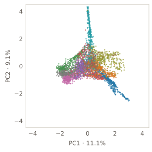
EpiJEPAEpiplexity + view agreement

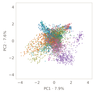
SIGRegGaussian regularisation + view agreement

Tench Spaniel Cassette Chainsaw Church Horn Truck Pump Golf ball Parachute

Introduction

JEPA methods are an important part of self-supervised learning. In the image-based setting explored here, they use an invariance objective to learn robust feature representations: an encoder embeds different views of the same object, and the objective pushes those embeddings to agree. Ideally, this preserves the pertinent “slow features” that remain stable across views, while discarding incidental detail.

In practice, view agreement alone admits a trivial solution: map every input to the same embedding. Regularisation steers optimisation away from this collapse and gives the encoder a reason to preserve useful variation.

In LeJEPA, SIGReg provides that anti-collapse mechanism, and it works very well. It also pushes the distribution of embeddings across a batch towards a Gaussian. A more elegant mechanism might measure the structured information in the embeddings directly and reward the encoder for preserving it. This led me to ask:

Can we use epiplexity to prevent collapse in JEPA embeddings?

Theory

What is epiplexity?

We can view epiplexity as a measure of the structured content in data that a learner can discover within a fixed compute budget.

The formal definition uses compression: find a model that makes the model itself and the data it describes as compact as possible, within that budget. Epiplexity is the number of bits needed to describe the resulting model, representing the structure it has captured.

A learning curve gives us one way to approximate this. As the learner picks up patterns, its prediction loss falls. The area above the final loss adds up how much worse its predictions were during learning than at the end. This area estimates the information acquired along the way; the final loss reflects what remains unexplained. Try changing the mixture below:

Tractable epiplexity calculation

To score embeddings at each training step, EpiJEPA uses a different approximation from Yanbo Zhang and Michael Levin's Intelligence from Learnable Novelty, based on a small predictor.

I pass the images through a fixed random feature extractor, called a reservoir. Then I fit a linear predictor, called a ridge readout, to predict the embeddings from those features. If the embeddings preserve several independent patterns from the images, the predictor may need several independent directions to represent them. A log-determinant score measures the strength and spread of those directions, approximating the predictor's description length.

This connects directly to collapse. If every embedding is identical, there is no variation for the predictor to explain: after centring, its weights and score are zero. Rewarding the score alongside view agreement gives the encoder an incentive to preserve variation connected to the images, helping prevent the trivial collapse to a constant output.

Method

For Imagenette, I took the training code directly from the LeJEPA repository's minimal example. I kept the encoder, projector, augmentations, optimiser and training schedule fixed, and replaced SIGReg with the epiplexity-inspired score. This keeps the comparison focused on the anti-collapse mechanism. My SIGReg baseline reached 90.42% online probe accuracy, close to the authors' reported 90.7%, giving a check that the original recipe was reproduced.

With this swap, the training loop keeps LeJEPA's view-agreement loss and adds a ridge fit for each view:

R ← frozen_random_CNN(features=64)

for each batch of images:
  views ← augment(images)
  Z ← encoder(views)

  for each view v:
    H ← normalise(R(views[v]))  // centre and scale
    W ← ridge_fit(H, centre(Z[v]))
    scores[v] ← logdet_score(W)

  agreement ← mean((Z − mean_over_views(Z))²)
  loss ← (1 − λ) × agreement − λ × mean(scores) / S₀
  update_encoder(loss)  // backpropagate through the ridge fit

A regularisation weight controls how strongly the score competes with view agreement. I scale the score by its value at the start of training so that the weight is easier to interpret.

Results

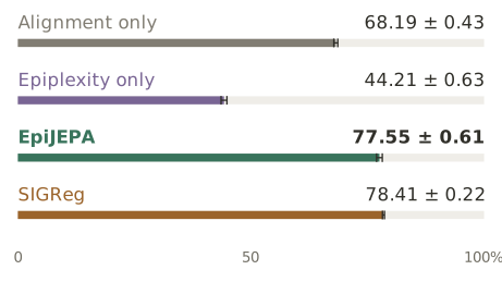
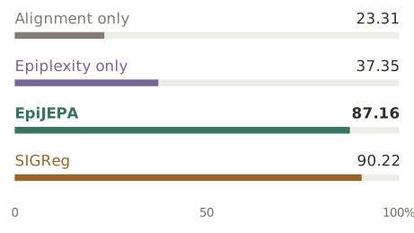
To assess what the encoder learns, I train a simple classifier on its features without letting the labels update the encoder. This is the probe accuracy shown below.

On Imagenette, the probes use backbone features before the projector. I also tested the projector outputs: accuracy was lower, but the gap between EpiJEPA and SIGReg stayed about the same.

CIFAR-10

Validation split · ResNet-18 · 3 seeds

Imagenette

Validation split · ViT-S/8 · 1 seed

Regularisation weight sweeps

CIFAR-10 · validation

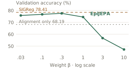
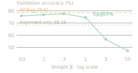
Imagenette · online probe

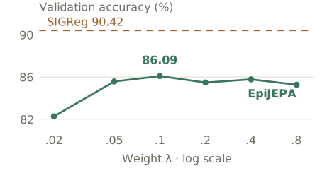
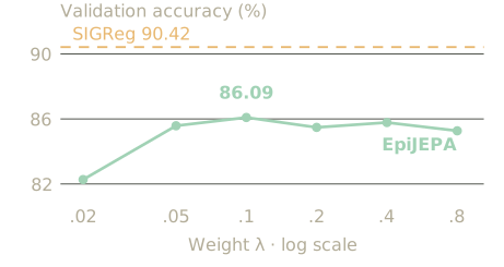
Imagenette · frozen probe

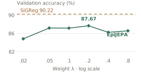
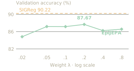
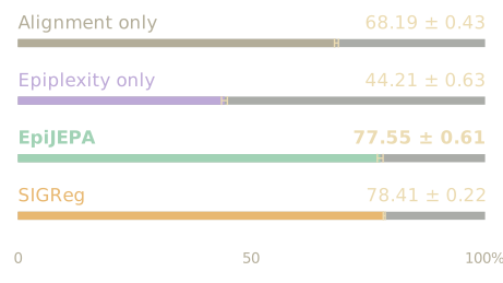
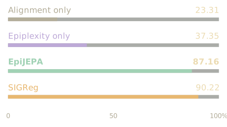
CIFAR error bars show one standard deviation across three seeds. Imagenette uses one seed, with SIGReg at λ = 0.02. Online probes train alongside the encoder; frozen probes are fitted afterwards. Sweep accuracy axes are cropped.

The repository contains both figures and the full result tables.

Conclusion

EpiJEPA can act as an anti-collapse mechanism in JEPA methods without imposing a specific embedding distribution. The Imagenette analysis supports this distinction: excess kurtosis is 3.41 for EpiJEPA and 0.14 for SIGReg, where a Gaussian has zero excess kurtosis.

EpiJEPA also uses more of the embedding space on CIFAR, with an effective rank of 58.4 versus 24.7 for SIGReg out of 64 dimensions. On Imagenette, both are close to full rank, and EpiJEPA's PCA plot looks more cleanly clustered to me. Yet these properties do not translate into better classification: its probe accuracy trails SIGReg by about one percentage point on CIFAR and three on Imagenette.

Removing view agreement substantially weakens classification. Epiplexity can prevent collapse on its own, but these results suggest it is insufficient as a standalone learning objective. View agreement helps turn that variation into useful semantic representations.

I think this method shows promise. I spent relatively little time refining the epiplexity implementation, so further tuning may help close the remaining accuracy gap to SIGReg.

Comments